library(brms) # Software for fitting Bayesian models
library(rstan)
library(ggplot2) # These two packages are for plotting
library(ggthemes)

# Loading in the data for all examples
load("data/MALD_subset.Rda")

# Setting global plotting theme
theme_set(
  theme_bw(base_size = 15) +
    theme(panel.grid.minor = element_blank(),
          panel.grid.major = element_line(color = "grey50",
                                          linetype = 2),
          legend.position = "none")
)

# Setting the seed for replicability
set.seed(101)
Setting priors for Bayesian analyses of reaction times in psycholinguistic experiments
Companion code
This is companion code to my talk at the EUTOPIA Methodological Workshop that is taking place as a satellite event to Giornate Italiane di Linguistica Sperimentale. My talk is meant to be more theoretical and conceptual in nature, but for those of you who are interested in how to conduct a prior predictive check in brms, you will find the basic code needed here along with brief explanations.
Setting up environment and loading data
Setting priors
Creating some convenience functions
Here we create two simple functions to save ourselves some typing later. The first one, prior_plot(), plots a number of simulated datasets based on our prior model. The second one, prior_samples(), gets a vector of the actual predicted reaction times from our prior model.
# This one plots priors
prior_plot <- function(model_fit, ...) {
  p <- pp_check(model_fit, ...)
  p$data <- p$data[p$data$is_y == FALSE,]
  p
}

# This one gets prior samples
prior_samples <- function(model_fit, ...) {
  p <- pp_check(model_fit, ...)
  p$data <- p$data[p$data$is_y == FALSE,]
  return(p$data$value)
}
Our first attempt at setting priors
For our first model, we talked a little bit about different possible priors and saw that they all made sense (more or less) in isolation. The first two lines show the model formula, and the last three specify the priors.
\(rt \sim Normal(\mu,\sigma)\)
\(\mu = \beta_0 + \beta_1 Frequency\)
\(\beta_0 \sim Normal(1000, 250)\)
\(\beta_1 \sim Normal(0, 200)\)
\(\sigma \sim Normal_+(0, 500)\)
Fitting our first set of priors
Here we save the priors above as a vector to use them in our model.
# Setting up a first set of priors
first_priors <- c(
  prior(normal(1000, 250), class = "Intercept"),
  prior(normal(0, 200), class = "b", coef = "sl_Freq"),
  prior(normal(0, 500), class = "sigma")
)
Now that we’ve saved our priors, we “fit” our model. The argument sample_prior = "only" means that the model will ignore our data, and just use our priors to create a the model object. In running this code for yourself, it doesn’t really matter what your data looks like, as long as you have a dataframe called dRT and the variables RT and sl_Freq this should run.
model_one <- brm(
  RT ~ sl_Freq, # model formula
  data = dRT, # pass the dataframe
  prior = first_priors, # pass our priors
  sample_prior = "only", # fit model using only priors
  cores = 4,
  control = list(adapt_delta = 0.95),
  file = "models/model_one.rds"
)
Visuzalizing twenty simulated datasets from our first priors
Here we use the prior_plot() function we created to simulate twenty different datasets based only on our priors. Changing the number of draws (ndraws) to a different number of simulated datasets.
# Making the plot
p1 <- prior_plot(model_one, ndraws = 20)

# Printing the plot with some minor changes
p1 +
  xlim(-2000, 5000) +
  labs(
    y = "density",
    x = "Reaction times (ms)"
  )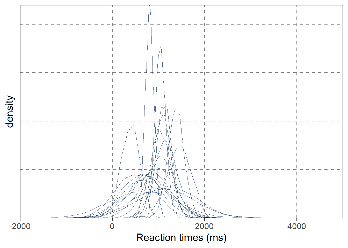
Getting quantiles of the reaction times
We can also use a combination of our prior_samples() function together with the quantile() function to look at the distribution of our data. Here we look at the median (0.50) along with the 1%, 5%, 95%, and 99% quantiles of our data.
quantile(prior_samples(model_one, ndraws = 100), probs = c(0.01, 0.05, 0.50, 0.95, 0.99)) 1% 5% 50% 95% 99%
-804.756002 1.135078 945.684071 1929.392243 2650.346405 A second attept: narrowing our priors
After seeing that our priors had too many fast (and impossible) reaction times, we then fit a model where we kept the measure of central tendency but changed the scale parameters (standard deviations) to be more narrow in order to make it so we don’t have as many negative values.
\(rt \sim Normal(\mu,\sigma)\)
\(\mu = \beta_0 + \beta_1 Frequency\)
\(\beta_0 \sim Normal(1000, 200)\)
\(\beta_1 \sim Normal(0, 100)\)
\(\sigma \sim Normal_+(0, 250)\)
second_priors <- c(
  prior(normal(1000, 200), class = "Intercept"),
  prior(normal(0, 100), class = "b", coef = "sl_Freq"),
  prior(normal(0, 250), class = "sigma")
)
Now that we have the new priors, we fit the model again.
model_two <- brm(
  RT ~ sl_Freq,
  data = dRT,
  prior = second_priors,
  sample_prior = "only",
  cores = 4,
  control = list(adapt_delta = 0.95),
  file = "models/model_two.rds"
)
We can plot the prior check again.
# Creating the plot
p2 <- prior_plot(model_two, ndraws = 20)

# Printing it with some minor changes
p2 +
  xlim(-2000, 5000) +
  labs(
    y = "density",
    x = "Reaction times (ms)"
  )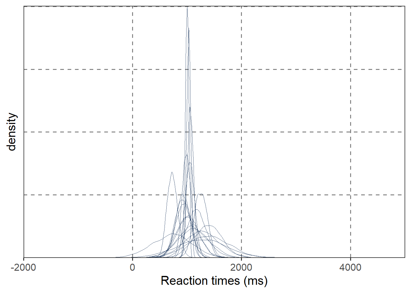
Getting quantiles of the reaction times
And we show the quantiles again.
quantile(prior_samples(model_two, ndraws = 100), probs = c(0.01, 0.05, 0.50, 0.95, 0.99)) 1% 5% 50% 95% 99%
108.1953 447.0236 1024.1208 1552.1931 1902.8835 A lognormal model of reaction times
We discussed in the presentation that a lognormal model of reaction times makes more sense given reaction times. Now we have a new model of reaction times to create priors for, but the model parameters we need priors for is the same. They are now on the log scale.
# Creating vector of priors in the log space
third_priors <- c(
  prior(normal(6.9, 0.25), class = "Intercept"),
  prior(normal(0, 0.1), class = "b", coef = "sl_Freq"),
  prior(normal(0, 0.5), class = "sigma")
)
Fitting the the lognormal model with only our priors. Notice that we now have a new argument, family = lognormal() which changes the likelihood function of our model. This actually changes a number of assumptions in our model which we didn’t have time to go into, but it is fairly well-suited to modelling reaction times.
model_three <- brm(
  RT ~ sl_Freq,
  data = dRT,
  family = lognormal(),
  prior = third_priors,
  sample_prior = "only",
  cores = 4,
  control = list(adapt_delta = 0.99),
  file = "models/model_three.rds"
)
Creating the prior plot
Again, we simulate twenty datasets from our priors to check our assumptions.
p3 <- prior_plot(model_three, ndraws = 20)

p3 +
  xlim(0, 5000) +
  labs(
    y = "density",
    x = "Reaction times (ms)"
  )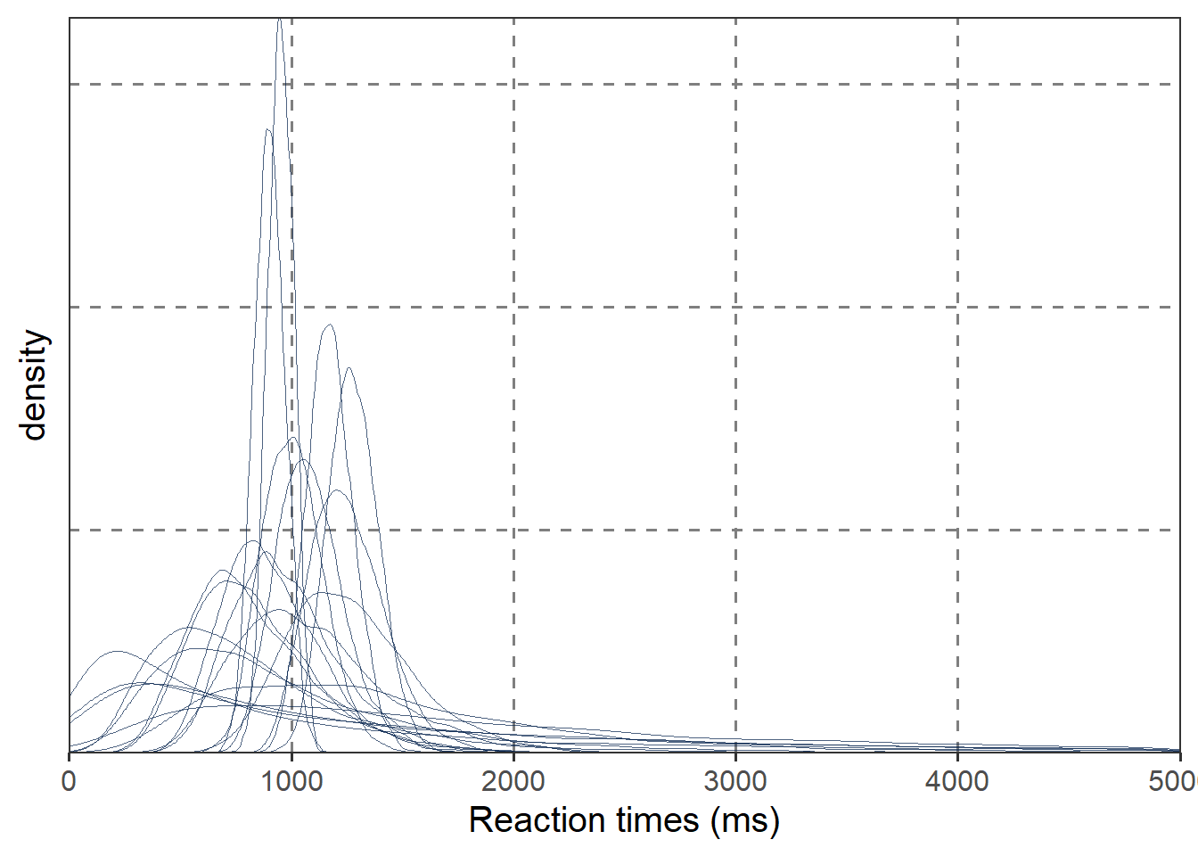
Getting quantiles of the reaction times
Checking the quantiles, we see that they make a lot more sense for our assumptions about the data.
quantile(prior_samples(model_three, ndraws = 100), probs = c(0.01, 0.05, 0.50, 0.95, 0.99)) 1% 5% 50% 95% 99%
220.5228 421.8860 983.1498 2418.3574 4344.8047